In the first subsection we introduce notation and present conjugate exponential family and latent variable models (LVMs). In the second subsection, we detail how to apply variational inference methods to fit LVMs from data. Finally, we show how to scale variational methods to learn LVMs over massive data sets.

Latent Variable Models

The conjugate exponential family [@barndorff2014information] has been largely studied in the statistics field and cover a very wide and widely used range of probability distributions and density functions such as Multinomial, Normal, Gamma, Dirichlet, Beta, etc. They have been largely used by the machine learning community [@bishop2006pattern; @koller2009probabilistic; @murphy2012machine] to exploit many of their nice properties for parameter learning and inference tasks.

[]

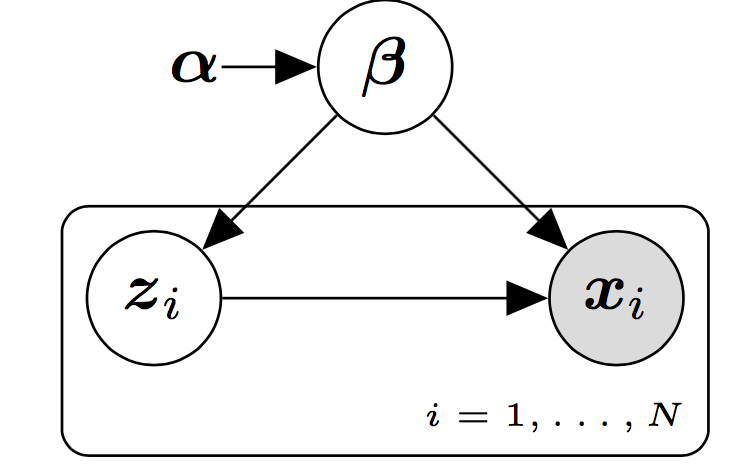
In our case, we focus on probabilistic models in Figure [fig:basemodel] with the structure shown in belonging to the conjugate exponential family. These kind of models are also known as latent variable models (LVMs) [@bishop1998latent; @blei2014build]. LVMs are widely used probabilistic models which tries to uncover hidden patterns in our data set. Usually, we are interested in local hidden patterns which are specific for every sample of our data as well as global hidden patterns that are shared among all the samples of the data set. These hidden patterns are explicitly modelled by means of a set of global, denoted by $\bmbeta$, and local stochastic random variables, denoted by $\bmz$, which can not be observed. The observed data, denoted by $\bmx$, is assumed to be generated from stochastic random variables whose distribution is conditioned to both the local and global hidden variables. A vector of fixed (hyper) parameters denoted by $\bmalpha$ is also included in this kind of models.

LVMs include popular models like LDA models to uncover the hidden topics in a text corpora [@blei2003latent], mixture of Gaussian models to discover hidden clusters in our data [@bishop2006pattern], probabilistic principal component analysis for revealing a low-dimensional representation of the data [@tipping1999probabilistic], models to capture the drift in a data stream [@masegosa2017bayesian], etc. And they have been used for knowledge extraction from GPS data [@kucukelbir2017automatic], genetic data [@pritchard2000inference], graph data [@kipf2016variational], etc. Many books contain entire sections devoted to them [@bishop2006pattern; @koller2009probabilistic; @murphy2012machine].

The joint distribution of this probabilistic model factorizes into a product of local terms and a global term,

[] \(p(\bmx, \bmz, \bmbeta) = p(\bmbeta) \prod_{i=1}^N p(\bmx_i, \bmz_i|\bmbeta).\)

As the model is assumed to belongs to the conjugate exponential family, the functional form of the conditional distributions of the model are specified as follows,

[] \(\begin{aligned} \ln p(\bmbeta) &=& \ln h(\bmbeta) + \bmalpha^T t(\bmbeta) - a_g(\bmalpha)\nonumber\\ \ln p(\bmz_i|\bmbeta) &=& \ln h(\bmz_i) + \eta_z(\bmbeta)^T t(\bmz_i) - a_z(\eta_z(\bmbeta))\nonumber\\ \ln p(\bmx_i|\bmz_i,\bmbeta) &=& \ln h(\bmx_i) + \eta_x(\bmz_i,\bmbeta)^T t(\bmx_i) - \eta_x(\bmz_i,\bmbeta)),\end{aligned}\)

where the scalar functions $h(\cdot)$ and $a_l(\cdot)$ are the base measure and the log-normalizer, respectively; the vector function $\bmt(\cdot)$ is the sufficient statistics vector.

By using properties of the conjugate exponential family, we can also derived the functional form of the joint distributions over the local variables $(\bmz_i,\bmx_i)$ given the global parameters $\bmbeta$,

[] \(\label{eq:jointexponentialform} \ln p(\bmx_i,\bmz_i|\bmbeta) = \ln h(\bmx_i,\bmz_i) + \bmbeta^{T} t(\bmx_i,\bmz_i) - a_l(\bmbeta),\)

Another standard assumption [@HoffmanBleiWangPaisley13] in this kind of models is that the complete conditional forms of the latent variables given the observations and the other latent variables can also be expressed in exponential family form,

[] \(\label{eq:posteriorexponentialform} \begin{split} \ln p(\bmbeta|\bmx, \bmz) = h(\bmbeta) + \eta_g(\bmx, \bmz)^T t(\bmbeta) - a_g(\eta_g(\bmx, \bmz))\\ \ln p(\bmz_i|\bmx_i, \bmbeta) = h(\bmz_i) + \eta_l(\bmx_i,\bmbeta)^T t(\bmz_i) - a_l(\eta_l(\bmx_i,\bmbeta)). \end{split}\)

By conjugacy properties, the natural parameter of the global posterior $\eta_g(\bmx, \bmz)$ can be expressed as, \(\label{eq:naturalglobal} \eta_g(\bmx, \bmz) = \bmalpha + \sum_{i=1}^N t(\bmx_i,\bmz_i)\)

[]

Example 1: Principal Component Analysis

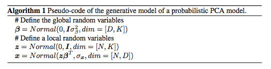
Principal Component Analysis (PCA) is a classic statistical technique for dimensionality reduction. It maps a D-dimensional point $\bmx$ to a K-dimensional latent representation $\bmz$ through a affine matrix $\bmbeta$ of dimensions $K\times D$. A simplified probabilistic view of PCA [@tipping1999probabilistic] can be describe as follows,

[] \(\label{eq:pca} \begin{aligned} %\bmalpha = (\sigma_\beta, \sigma_z, \sigma_x)\nonumber\\ \bmbeta \sim \calN_{d\times k} (0,\bmI\sigma^2_\beta) \nonumber\\ \bmz_i \sim \calN_k (0,\bmI)\nonumber\\ \bmx_i \sim \calN_d (\bmbeta^T\bmz_i, \bmI\sigma^2_x ), \end{aligned}\)

where $\bmalpha = (\sigma^2_\beta, \sigma^2_x)$ are the hyperparameters of the model.

Algorithm [alg:pca] provides a pseudo-code a description of the generative model of a probabilistic PCA model.

[]

This model is a LVM where $\bmbeta$ acts a the global hidden variable and $\bmz_i$ is the local hidden variables associated to the sample $\bmx_i$. It belongs to the conjugate exponential family because all the conditionals are Gaussian distributions whose the mean is expressed as a linear combination of preceding variables [@koller2009probabilistic]. Therefore, they satisfy Equation ([eq:model].

Note that this linear relationship between the hidden and the observed variables is a strong limitation of this model [@scholkopf1998nonlinear]. Also note this linear relationship is made to guarantee that the model belongs to conjugate exponential family. The use of any other non-linear relationship would make the PCA model to not belong to this family and would prevent, as we will see in the next post, the use of efficient inference algorithms. Something similar happens with the variance parameter $\sigma_x$, which can not depend on the latent variables $\bmz_i$ in order to belong to the conjugate exponential family.

LVMs include popular models like LDA models [@blei2003latent] to uncover the hidden topics in a text corpora, mixture of Gaussian models to discover hidden clusters in our data [@bishop2006pattern], probabilistic principal component analysis for revealing a low-dimensional representation of the data [@tipping1999probabilistic], models with hierarchical latent variables to capture the drift in a data stream [@borchani2015modeling; @masegosa2017bayesian], etc. Many machine-learning books contain entire sections devoted to them [@bishop2006pattern; @koller2009probabilistic; @murphy2012machine].

Mean-Field Variational Inference

The problem of Bayesian inference reduces to compute the posterior over the unknown quantities (i.e. the global and local hidden variables $\bmbeta$ and $\bmz$, respectively) given the observations,

[] \(\label{eq:VI} p(\bmbeta, \bmz\given \bmx) = \frac{p(\bmx|\bmz,\bmbeta)p(\bmz\given \bmbeta)p(\bmbeta)}{\int p(\bmx|\bmz,\bmbeta)p(\bmz\given \bmbeta)p(\bmbeta) d\bmz d\bmbeta}.\)

Computing the above posterior is usually intractable for many interesting models because it requires to solve a highly-multidimensional integral. As commented in the in the introduction, VI methods are one of the best performing options to address this problem. In this post we revise the main ideas behind this approach.

Variational inference is a deterministic technique for finding tractable posterior distributions, denoted by $q$, which approximates the Bayesian posterior, $p(\bmbeta,\bmz|\bmx)$, that is often intractable to compute. More specifically, by letting ${\cal Q}$ be a set of possible approximations of this posterior, variational inference solves the following optimization problem for any model in the conjugate exponential family:

[] \(\label{eq:VIKL} \min_{q\left(\bmbeta,\bmz\right)\in {\cal Q}} \KL(q(\bmbeta,\bmz)||p(\bmbeta,\bmz|\bmx)),\)

where $\KL$ denotes the Kullback-Leibler divergence between two probability distributions.

In the mean field variational approach the approximation family ${\cal Q}$ is assumed to fully factorize. Following the notation of @HoffmanBleiWangPaisley13, we have that

[] \(q(\bmbeta,\bmz\given \bmlambda,\bmphi) = q(\bmbeta \given \bmlambda)\prod_{i=1}^N q(\bmz_i \given \bmphi_i).\)

where $\bmlambda$ parameterizes the variational distribution of $\bmbeta$, while $\bmphi$ has the same role for the variational distribution of $\bmz$

Furthermore, each factor in the variational distribution is assumed to belong to the same family of the model’s complete conditionals (see Equation [eq:posteriorexponentialform],

[] \(\label{eq:qexponentialform} \begin{split} \ln q(\bmbeta|\bmlambda) = h(\bmbeta) + \bmlambda^T t(\bmbeta) - a_g(\bmlambda)\\ \ln q(\bmz_i|\bmphi_i) = h(\bmz_i) + \bmphi_i^T t(\bmz_i) - a_l(\bmphi_i). \end{split}\)

To solve the minimization problem in Equation ([eq:VI], the variational approach exploits the transformation

[] \(\label{eq:likelihood_decomposition} \ln p(\bmx) = {\cal L}(\bmlambda,\bmphi) + \KL(q(\bmbeta,\bmz\given \bmlambda,\bmphi)||p(\bmbeta,\bmz|\bmx)),\)

where ${\cal L}(\cdot|\cdot)$ is a lower bound of $\ln P(\bmx)$ since $\KL$ is non-negative. As $\ln p(\bmx)$ is constant, minimizing the $\KL$ term is equivalent to maximizing the lower bound. Variational methods maximize this lower bound by using gradient based methods.

The functional form of the $\lb$ function can expressed as follows,

[] \(\label{eq:elbo} \begin{split} {\cal L}(\bmlambda,\bmphi) = & \E_q [\ln p(\bmx, \bmz, \bmbeta)] - \E_q [\ln q(\bmbeta,\bmz|\bmlambda,\bmphi)]\\ \end{split}\)

The key advantage of having a conjugate exponential model is that the gradients of the $\lb$ function can be always computed in closed form  [@WinnBishop05]. The gradients with respect to the variational parameters $\bmlambda$ and $\bmphi$ can be computed as follows,

[] \(\label{eq:gradELBO} \begin{split} \nabla^{nat}_\lambda {\cal L} (\bmlambda,\bmphi) &= \bmalpha + \sum_{i=1}^N \E_{\phi_i} [t(\bmx_i,\bmz_i)] - \bmlambda\\ \nabla^{nat}_{\phi_i}{\cal L} (\bmlambda,\bmphi) &= \E_\lambda [\eta_l(\bmx_i,\bmbeta)] - \bmphi_i, \end{split}\)

where $\nabla^{nat}$ denotes natural gradients[^1], and $\E_{\phi_i}[\cdot]$ and $\E_\lambda [\cdot]$ denote expectations with respect to $q(\bmz_i\given\bmphi_i)$ and $q(\bmbeta\given\bmlambda)$, respectively.

From the above gradients we can derive a coordinate ascent algorithm to optimize the ELBO function with the following coordinate ascent rules,

[] \(\begin{aligned} \label{eq:CoordinateAscent} \bmlambda^\star &=& \arg\max_{\lambda} {\cal L} (\bmlambda, \bmphi) = \bmalpha + \sum_{i=1}^N \E_{\phi_i} [t(\bmx_i,\bmz_i)] \nonumber\\ \bmphi_i^\star &=& \arg\max_{\phi_i} {\cal L} (\bmlambda, \bmphi) = \E_\lambda [\eta_l(\bmx_i,\bmbeta)].\end{aligned}\)

By iteratively running the above updating equations, we are guranteed to (i) monotonically increased the ELBO function at every time step and (ii) to converge to stationary point of the ELBO function or, equivalently, the minimization function of Equation [eq:VIKL].

[]

Example 2: Variational Inference over the PCA model

For the PCA model depicted in Example [example:PCA], the variational distributions would be,

[] \(\begin{aligned} q(\bmbeta\given \bmmu_{\beta}, \mathbf{\Sigma}_{\beta}) = {\cal N}_{d\times k}(\bmmu_{\beta}, \mathbf{\Sigma}_{\beta})\\\\ q(\bmz_i\given \bmmu_{z,i}, \mathbf{\Sigma}_{z,i}) = {\cal N}_{k}(\bmmu_{z,i}, \mathbf{\Sigma}_{z,i})\end{aligned}\)

Given the above variational family, the coordinate updating equations derived from Equation [eq:CoordinateAscent] can be written as follows [@bishop2006pattern],

[] \(\begin{aligned} \bmmu_{\beta}^\star &=& \big[\sum_{i=1}^N (\bmx_i - \bar{\bmx})\E[\bmz_i]^T\big]\mathbf{\Sigma}_{\beta}\\ \mathbf{\Sigma}_{\beta}^\star &=& \sum_{i=1}^N \E[\bmz_i\bmz_i^T] + \sigma_x A\\ \bmmu_{z,i}^\star &=& \sigma_x^2 \mathbf{\Sigma}_{z,i}^{-1}\bmmu_{\beta}^T(\bmx_i -\bar{\bmx})\\ \mathbf{\Sigma}_{z,i}^\star &=& \sigma_x^{-2}\bmmu_{\beta}^T\bmmu_{\beta} + \bmI\end{aligned}\)

where $A$ is a diagonal matrix with elements $\alpha_i = \frac{d}{\bmmu_{\beta,i}^T\bmmu_{\beta,i}}$. Again, we have a nice set of close-form equations which guarantees convergence to the solution of the inference problem. But we should note that this is possible due to the strong assumptions imposed to the probabilistic model and to the variational approximation family. —

Scalable Varitional Inference

Performing variational inference in big data sets (i.e. when N is a very large number) raises many challenges. Firstly, the model itself may not fit in memory, and, secondly, computing the ELBO’s gradient wrt $\bmlambda$ depends linearly on the size of the data set (see Equation [eq:gradELBO], which can be prohibitively expensive in this case. Stochastic Variational inference (SVI) [@HoffmanBleiWangPaisley13] is the most popular method for scaling VI to massive data sets, and relies on stochastic optimization techniques [@bottou2010large; @robbins1951stochastic].

We start reparamerizing the ELBO’s function ${\cal L}$ only in terms of the variational global parameters $\bmlambda$, by defining, \(\label{eq:scalable:elbo} {\cal L}(\bmlambda) = {\cal L}(\bmlambda,\bmphi^\star(\bmlambda))\) where $\bmphi^\star(\bmlambda)$ is defined as in Equation [eq:CoordinateAscent], i.e. it returns a local optimum of the local variational parameters for a given $\bmlambda$. By using the equality

[] \(\nabla^{nat}_\lambda {\cal L}(\bmlambda) = \nabla^{nat}_\lambda {\cal L}(\bmlambda,\bmphi^\star(\bmlambda))\)

[@HoffmanBleiWangPaisley13], the natural gradient wrt $\bmlambda$ can be computed as follows,

[] \(\label{eq:scalable:gradient} \nabla^{nat}_\lambda {\cal L}(\bmlambda) = \bmalpha + \sum_{i=1}^N \E_{\phi^\star} [t(\bmx_i,\bmz_i)] - \bmlambda\\\)

The key idea behind the stochastic variational method is to compute noise and unbiased estimates of the ELBO’s gradient, denoted by $\hat{\nabla}^{nat}_\lambda {\cal L}$, by randomly selecting a mini-batch of $M$ data samples,

[] \(\label{eq:scalable:gradientNoisy} \begin{split} \hat{\nabla}^{nat}_\lambda {\cal L} (\bmlambda) = \bmalpha + \frac{N}{M}\sum_{m=1}^M \E_{\phi^\star_i} [t (\bmx_{i_m},\bmz_{i_m})] - \bmlambda, \end{split}\)

where $i_m$ is the variable index form the subsampled mini-batch. This is an unbiased estimate because \(\E[\hat{\nabla}^{nat}_\lambda {\cal L}] = \nabla^{nat}_\lambda {\cal L}\).

According to stochastic optimization theory [@robbins1951stochastic], the ELBO can be maxizimed by following noisy estimates of the gradient,

[] \(\label{eq:gradELBONoisy} \begin{split} \bmlambda^{t+1} = \bmlambda^t + \rho_t \hat{\nabla}^{nat}_\lambda {\cal L}(\bmlambda^t), \end{split}\)

if the learning rate $\rho_t$ satisfies the Robbins-Monro conditions (i.e. $\sum_{t=1}^\infty \rho_t = \infty$ and $\sum_{t=1}^\infty \rho^2_t<\infty$), and the above updating equation is guarantee to converge to a stationary point of the ELBO function.

The size of the mini-batch is chosen to be $M«N$ to reduce the computational complexity of computing the gradient, and with $M>1$ in order to reduce the variance in the estimate of the gradient. The optimal value is used to be problem dependent [@li2014efficient].

Alternative ways to scale up variational inference in conjugate exponential models involve the use of distributed computing clusters. For example, in [@masegosa2017scaling] the data set is assumed to be stored among different machines. Then the problem of computing the ELBO’s gradient given in Equation [eq:gradELBO] is scaled up by distributing the computation of the gradient \(\nabla^{nat}_{\phi_i}{\cal L} (\bmlambda,\bmphi)\). So each machine computes this term for those samples that are locally stored. Finally, all the terms are sent to a master node which aggregates them and compute the gradient $\nabla^{nat}_\lambda {\cal L} (\bmlambda,\bmphi)$ (see Equation [eq:gradELBO]).

References

Amari, Shun-Ichi. 1998. “Natural Gradient Works Efficiently in Learning.” Neural Computation 10 (2): 251–76.
Barndorff-Nielsen, Ole. 2014. Information and Exponential Families: In Statistical Theory. John Wiley & Sons.
Bishop, Christopher M. 1998. “Latent Variable Models.” In Learning in Graphical Models, 371–403. Springer.
———. 2006. Pattern Recognition and Machine Learning. springer.
Blei, David M. 2014. “Build, Compute, Critique, Repeat: Data Analysis with Latent Variable Models.” Annual Review of Statistics and Its Application 1: 203–32.
Blei, David M, Andrew Y Ng, and Michael I Jordan. 2003. “Latent Dirichlet Allocation.” Journal of Machine Learning Research 3 (Jan): 993–1022.
Borchani, Hanen, Ana M Martı́nez, Andrés R Masegosa, Helge Langseth, Thomas D Nielsen, Antonio Salmerón, Antonio Fernández, Anders L Madsen, and Ramón Sáez. 2015. “Modeling Concept Drift: A Probabilistic Graphical Model Based Approach.” In International Symposium on Intelligent Data Analysis, 72–83. Springer.
Bottou, Léon. 2010. “Large-Scale Machine Learning with Stochastic Gradient Descent.” In Proceedings of Compstat’2010, 177–86. Springer.
Hoffman, Matthew D., David M. Blei, Chong Wang, and John Paisley. 2013. “Stochastic Variational Inference.” Journal of Machine Learning Research 14: 1303–47.
Kipf, Thomas N, and Max Welling. 2016. “Variational Graph Auto-Encoders.” arXiv Preprint arXiv:1611.07308.
Koller, Daphne, and Nir Friedman. 2009. Probabilistic Graphical Models: Principles and Techniques. MIT press.
Kucukelbir, Alp, Dustin Tran, Rajesh Ranganath, Andrew Gelman, and David M Blei. 2017. “Automatic Differentiation Variational Inference.” The Journal of Machine Learning Research 18 (1): 430–74.
Li, Mu, Tong Zhang, Yuqiang Chen, and Alexander J Smola. 2014. “Efficient Mini-Batch Training for Stochastic Optimization.” In Proceedings of the 20th Acm Sigkdd International Conference on Knowledge Discovery and Data Mining, 661–70. ACM.
Masegosa, Andrés, Thomas D Nielsen, Helge Langseth, Dario Ramos-Lopez, Antonio Salmerón, and Anders L Madsen. 2017. “Bayesian Models of Data Streams with Hierarchical Power Priors.” arXiv Preprint arXiv:1707.02293.
Masegosa, Andrés R, Ana M Martinez, Helge Langseth, Thomas D Nielsen, Antonio Salmerón, Darı́o Ramos-López, and Anders L Madsen. 2017. “Scaling up Bayesian Variational Inference Using Distributed Computing Clusters.” International Journal of Approximate Reasoning.
Murphy, Kevin P. 2012. Machine Learning: A Probabilistic Perspective. MIT press.
Pritchard, Jonathan K, Matthew Stephens, and Peter Donnelly. 2000. “Inference of Population Structure Using Multilocus Genotype Data.” Genetics 155 (2): 945–59.
Robbins, Herbert, and Sutton Monro. 1951. “A Stochastic Approximation Method.” The Annals of Mathematical Statistics, 400–407.
Schölkopf, Bernhard, Alexander Smola, and Klaus-Robert Müller. 1998. “Nonlinear Component Analysis as a Kernel Eigenvalue Problem.” Neural Computation 10 (5): 1299–1319.
Tipping, Michael E, and Christopher M Bishop. 1999. “Probabilistic Principal Component Analysis.” Journal of the Royal Statistical Society: Series B (Statistical Methodology) 61 (3): 611–22.
Winn, John M., and Christopher M. Bishop. 2005. “Variational Message Passing.” Journal of Machine Learning Research 6: 661–94.
Natural gradient is the standard gradient permultiplied by the inverse of the Fisher information matrix. They advantage of these gradients is that they account for the Riemannian geometry of the parameter space (Amari 1998).↩