Artificial Neural Networks

An artificial neural network (ANN) can be seen as a deterministic non-linear function $f(\cdot: \bmw)$ parametrized by a parameter vector $\bmw$. A ANN with $L$ hidden layers define then a mapping from a given input $\bmx$ to a given output $\bmy$. This mapping is built by the recursive application of a sequence of non-linear transformations,

[] \(\begin{aligned} \label{eq:ANNs} \bmh_0 &=& a_0(\bmx\bmw_0^T)\nonumber\\ &\ldots &\nonumber\\ \bmh_{l} &=& a_l(\bmh_{l-1}\bmw_{l-1}^T)\nonumber\\ &\ldots &\nonumber\\ \bmy &=& a_L(\bmh_{L}\bmw_L^T)\end{aligned}\)

where $a_l(\cdot)$ defines the activation (non-linear) function at the $l$-th layer, usual activations functions include the soft-max or the relu functions. $\bmw_l$ are the parameters defining the linear transformation at the $l$-th. The dimension of $\bmw_0$, $\bmw_l$ and $\bmw_L$ matrix are equal to $[d_0,d_x]$, $[d_l,d_{l-1}]$ and $[1,d_L]$, respectively. Then, $d_x$ is the dimension of the input data and $d_l$ is the so-called number of hidden units at the $l$-th layer. DNNs is just a simple rename of classic ANNs, with the key difference than DNNs usually have a high number of hidden layers, much higher than classic ANNs used to have.

Fitting a DNN from a given data set of input-output pairs $(\bmx,\bmy)$ reduces to solve the following optimization problem,

[] \(\label{eq:dnnlearning} \bmw^\star = \arg\min_\bmw \sum_{i=1}^N \ell (y_i,f(\bmx_i;\bmw)),\)

where \(\ell (\bmy_i,\hat{\bmy}_i)\) is a loss function which defines a missmatch between the real output \(\bmy_i\) and produced output \(\hat{\bmy}_i = f(\bmx_i;\bmw)\) by the DNN model. This continuous optimization problem is usually solve by the application of a stochastic gradient descent method, or some of its famous variants, which involves the computation of the gradient of the loss function with respect to the parameters of the ANN, $\nabla_\bmw \ell (y_i,f(\bmx_i;\bmw))$. The algorithm for computing this gradient in a ANN is known as the back-propagation algorithm, which is based on the recursive application of the chain-rule of derivatives.

Computational Graphs

Computational graphs have been extremely useful when developing algorithms and software packages for neural networks and other models in machine learning [@chen2015mxnet; @abadi2016tensorflow; @paszke2017automatic]. The main idea of a computational graph is to express a (deterministic) function, as is the case of a neural network, as an acyclic directed graph defining a sequence of computational operations. A computational graph is composed by input nodes and operation nodes. Input nodes are set externally like the data sets, but also including the parameters we differentiate with respect to. Each operation node will be represented as squares in the subsequent diagrams; and each operation produces an output based on its inputs. The directed edges in the graph are used to specify those inputs to each node. Nodes are usually defined as tensors (n-dimensional arrays) and operations are then defined over these tensors too.

One of the strengths of computational graphs is that they allow to easily combine simple functions to form more complex functions: the vast majority of current neural networks can be defined using a computational graph.

But the key strength of computational graphs is that they allow for automatic differentiation. As shown in the previous post, most neural network learning algorithms translate to continuous optimization of a given differentiable loss function that is solved by gradient descent algorithms. Computational graphs allow to easily combine simple functions to form more complex functions: the vast majority of current loss functions involving neural networks can be defined using a computational graph. Automatic differentiation is a technique for automatically computing the derivatives of the function encoded by the computational graph: once the graph has been defined using underlying primitive operations, derivatives are automatically calculated based on the "local" derivatives of these operations. Before computational graphs were introduced in deep learning, those derivatives have to be computed manually, giving rise to a slow process quite prone to errors.

[]

Example 3: A simple artificial neural network

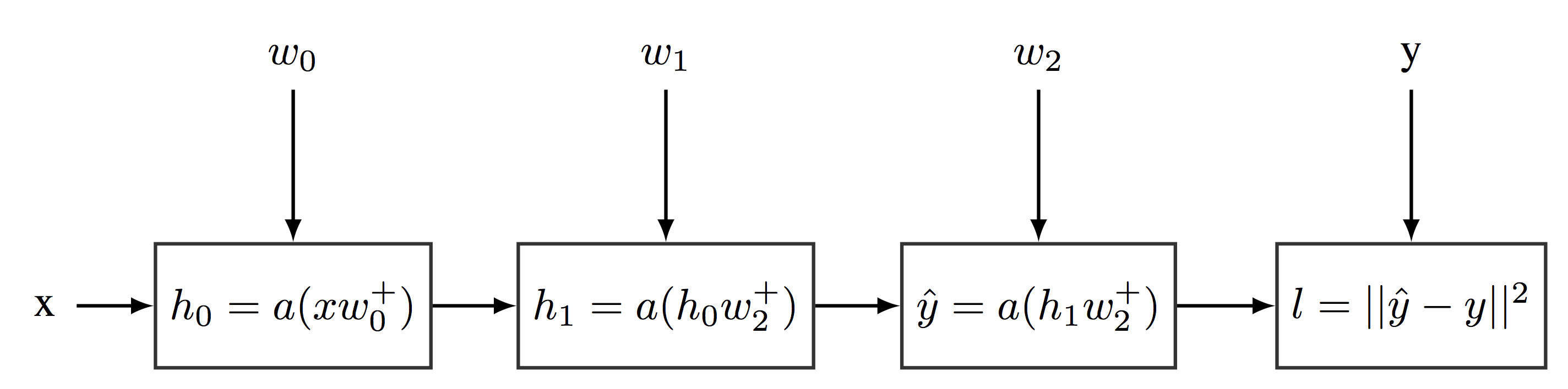[] Example of a Simple Computational Graph

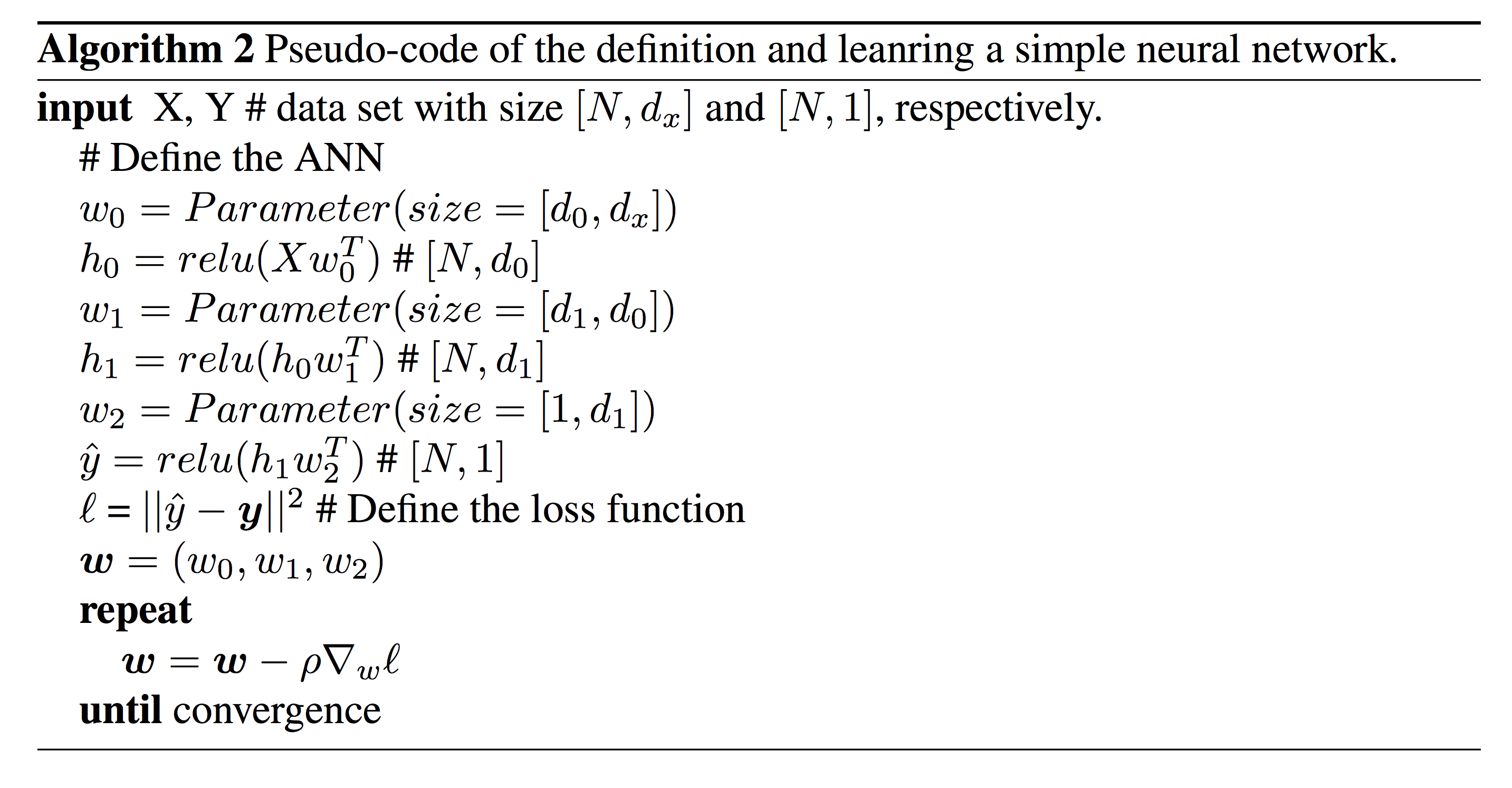
Figure [fig:computationalgraph] provides an example of a computational graph encoding a neural network with $\bmx$ as input, $\hat{\bmy}$ as output, and two hidden layers of 64 hidden units each. This computational graph also encodes the loss function $\ell(\bmy,\hat{\bmy})$. Even more, as computational graphs can be defined over matrixes (and tensors), the above computational graph can encode the application of the neural network over a whole training data set, or small mini-batch, $\bmx$ and, then, compute the loss function over these set of samples for a fixed vector of weights. Algorithm [alg:nn] shows the pseudo-code description for defining and learning this neural network. Note that gradients are automatically computed from the computational graph.

[]

References

Abadi, Martı́n, Paul Barham, Jianmin Chen, Zhifeng Chen, Andy Davis, Jeffrey Dean, Matthieu Devin, et al. 2016. “Tensorflow: A System for Large-Scale Machine Learning.” In OSDI, 16:265–83.
Chen, Tianqi, Mu Li, Yutian Li, Min Lin, Naiyan Wang, Minjie Wang, Tianjun Xiao, Bing Xu, Chiyuan Zhang, and Zheng Zhang. 2015. “Mxnet: A Flexible and Efficient Machine Learning Library for Heterogeneous Distributed Systems.” arXiv Preprint arXiv:1512.01274.
Paszke, Adam, Sam Gross, Soumith Chintala, Gregory Chanan, Edward Yang, Zachary DeVito, Zeming Lin, Alban Desmaison, Luca Antiga, and Adam Lerer. 2017. “Automatic Differentiation in Pytorch.”