Variational Inference with Deep Neural Networks

The variational inference problem of a probabilistic model with deep neural networks is again to maximize the ELBO function ${\cal L}(\bmlambda)$, which is equivalent to minimizing the KL divergence between the variational posterior and the target distribution. As we commented in the previous post when our probabilistic model contains complex constructs like DNNs, it falls outside the conjugate exponential family described and the variational inference methods described there do not apply here. In this post, we introduce the main methods employed to perform variational inference over probabilistic models containing deep neural networks.

Black Box Variational Inference

For the shake of simplicity, let us reparametrize the ELBO function with $\bmh=(\bmbeta,\bmz)$ and $\bmnu = (\bmlambda,\bmphi)$, and let us defined $g(\bmh,\bmnu) = \ln p(\bmx,\bmh) - \ln q(\bmh\given\bmnu)$. Then, the ELBO function ${\cal L}$ is expressed as follows,

[] \({\cal L}(\bmnu) = \E_q[g(\bmh,\bmnu)] = \int q(\bmh\given\bmnu) g(\bmh,\bmnu) d\bmh\)

This ELBO function can be easily represented in terms of a stochastic computational graph as shown in Figure [fig:ELBOSCG]. If we were dealing with standard CG, the optimization of this function would be straightforward thanks to the use of automatic differentiation. However, optimizing over SCGs is much more challenging because automatic differentiation does not readily apply. The main problem lies in computing the gradient of the ELBO function wrt $\bmnu$, which is a parameter affecting an expectation,

[] \(\label{eq:gradELBODNNs} \nabla_\bmnu {\cal L}= \nabla_\bmnu \E_{q}[g(\bmh,\bmnu)].\)

In the case of conjugate models, we could take advantage of their properties and derived closed-form solutions for this problem. But, in general, there are no closed-form solutions for computing gradients in non-conjugate models. See, for example, the case of a Bayesian logistic regression model [@murphy2012machine].

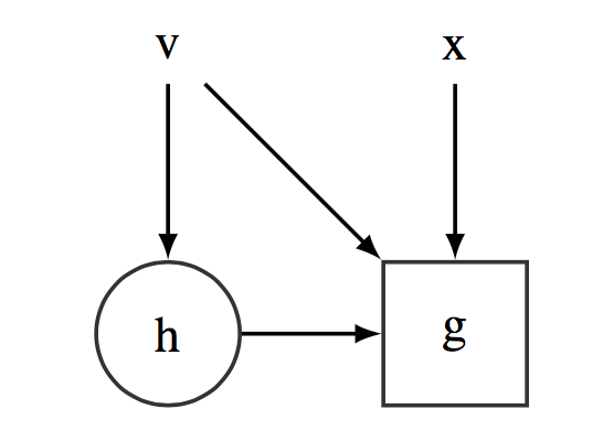[] Stochatic Computational Graph representing the ELBO function ${\cal L}(\bmnu)$. $\bmh$ is distributed according to the variational distribution, $\bmh \sim q(\bmh|\bmnu)$.

In this section, we provide two generic solutions for computing the gradient of the ELBO function for probabilistic models including DNNs, which directly rely on the automatic differentiation engines available for standards computational graphs. In that way, they extend the automatic differentiation methods of standard computational graphs to SCGs, giving rise to a powerful approach for variational inference on generic probabilistic models. The main idea of the following approaches is to compute the gradient of an expectation using Monte Carlo techniques. More precisely, we will show how we can build unbiased estimates of the gradient by sampling from the variational (or an auxiliary) distribution without having to compute the gradient of the ELBO analytically [@ranganath2014black; @wingate2013automated; @mnih2014neural].

Pathwise Graidents

The idea of this approach is to exploit reparametrizations of the variational distribution in terms of deterministic transformations of a noise distribution [@glasserman2013monte; @fu2006gradient]. A distribution $q(\bmh|\bmnu)$ is reparametrizable if it can be expressed as follows,

[] \(\label{eq:reparam} \begin{split} &\bmepsilon\sim q(\bmepsilon)\\ & \bmh = t(\bmepsilon; \bmnu) \end{split}\)

where $\bmepsilon$ does not depend of the $\bmnu$ parameter $t(\cdot; \bmnu)$ is a deterministic function which encapsulates the dependence of $\bmh$ with respect to $\bmmu$. This allows to compute any expectation over $\bmh$ as an expectation over $\bmepsilon$. Exploiting this reparametrization property we wan express the $\lb$’s gradient of Equation [eq:gradELBOGeneral] as follows [@kingma2013auto; @rezende2014stochastic; @titsias2014doubly],

[] \(\label{eq:gradELBOReparam} \begin{split} \nabla_\nu {\cal L}(\bmnu) &= \nabla_\nu \E_\nu [ g(\bmh,\bmnu)]\\ &=\nabla_\nu \E_\epsilon[ g(t(\epsilon; \bmnu),\bmnu)]\\ &= \E_\epsilon[ \nabla_\nu g(t(\epsilon; \bmnu),\bmnu)]\\ &= \E_\epsilon[ \nabla_h g(\bmh,\bmnu)^T\nabla_\nu t(\epsilon; \bmnu)]\\ \end{split}\)

Note that once we employ this reparametrization trick, the gradient can enter the expectation, something that could not happen with the score function gradient method. The key advantage of this method is that the gradient estimator is informed by the gradient with respect to $\bmh$, which gives the direction of the maximum posterior mode.

In terms of an SCG, this approach can be applied by transforming the original SCG described in Figure [fig:ELBOSCG] to the SCG described in Figure [fig:scgreparam]. Introducing this change, the underlying CG (as discussed in Figure [fig:EvaluatingStochasticCG]) can be readily applied and employ automatic differentiation to get unbiased estimates of the gradients of the ELBO.

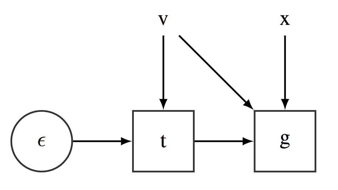[] Reparametrized Stochatic Computational Graph representing the ELBO function ${\cal L}(\bmnu)$. $\bmepsilon$ is distributed according to standard distribution, $\bmepsilon \sim q(\bmepsilon)$.

The Normal distribution is the best known example where this technique can be applied. I.e. A variable $\bmw\sim {\cal N} (\bmmu, \mathbf{\Sigma})$ can be reparametized as $\epsilon\sim {\cal N} (0, \bmI)$ and $\bmw = \bmmu + L\epsilon$ where $\mathbf{\Sigma}=LL^T$. The problem with this approach is that only a few distributions has this property [@kingma2013auto].

[@figurnov2018implicit] recently introduced an implicit reparametrization approach which apply to a wider range of distributions including Gamma, Beta, Dirichlet and von Misses. This method computes the $\lb$’s gradient as follows,

[] \(\label{eq:gradELBOImplicitReparam} \nabla_\nu {\cal L}(\bmnu) = - \E_\nu [ \frac{\nabla_h g(\bmh,\bmnu)^T\nabla_\nu F(\bmh; \bmnu)}{q(\bmh\given\bmnu)}],\)

where $F(\bmh; \nu)$ is the cumulative density function of $q(\bmh\given\nu)$. Other similar approaches has been proposed for models with discrete latent random variables [@tucker2017rebar; @grathwohl2017backpropagation].

This family of gradient estimators usually has lower variance than other methods [@kucukelbir2017automatic] and they can even get good estimates using a single Monte Carlo sample in many cases. By this algorithm requires the existence of the above (implicit) reparametrizations which do not cover many relevant distributions, as it is they case of the multinomial distribution. Additionally, this method also requires that both the log-joint distribution and the variational distributions are differentiable.

Score Function Gradients

This is a classic method for gradient estimation, also known as the REINFORCE gradient, [@ranganath2014black; @glynn1990likelihood; @williams1992simple]. This method builds on the following generic transformations to compute the gradient of an expected value,

[] \(\label{eq:gradELBOGeneral} \begin{split} \nabla_\nu {\cal L}(\bmnu) &= \nabla_\nu\int q(\bmh\given\bmnu) g(\bmh,\bmnu) d\bmh\\ & = \int \nabla_\nu q(\bmh\given\bmnu) g(\bmh,\bmnu) + q(\bmh\given\bmnu) \nabla_\nu g(\bmh,\bmnu)d\bmh\\ & = \int q(\bmh\given\bmnu) \nabla_\nu \ln q(\bmh\given\bmnu) g(\bmh,\bmnu)+ q(\bmh\given\bmnu) \nabla_\nu g(\bmh,\bmnu)d\bmh\\ &= \E_\nu [\nabla_\nu \ln q(\bmh\given\bmnu) g(\bmh,\bmnu) + \nabla_\nu g(\bmh,\bmnu)]. \end{split}\)

As $\E_\nu [\nabla_\nu g(\bmh,\bmnu)] = \E_\nu [\nabla_\nu \ln q(\bmh|\bmnu)] = 0$, the gradient of the ELBO simplifies to,

[] \(\label{eq:gradELBOScore} \nabla_\nu {\cal L}(\bmnu) = \E_\nu [\nabla_\nu\ln q(\bmh\given\bmnu) g(\bmh,\bmnu)].\)

From the above equation, we can obtain unbiased estimates of the gradient by sampling from $q(\bmh\given\bmnu)$. This method is pretty general because it only requires to evaluate the function $g(\bmh,\bmnu)$ and to compute the gradient for the variational approximation, $\nabla_\nu\ln q(\bmh\given\bmnu)$. In consequence, it applies to a really wide range of models including those ones already covered by pathwise gradients. However, this algorithm may easily suffer from high variance estimates of the gradients when the dimension of $\bmnu$ is relatively high. So, it may require to introduce variance reduction techniques to make it work successfully [@ruiz2016generalized; @ranganath2014black; @titsias2014doubly; @mnih2016variational]. In practical settings, one should only resort to this method when the pathwise gradients estimators are not applicable.

In terms of SCG, this trick can be nicely implemented following the indications given in [@foerster2018dice]. The main idea is to transform the computational graph is such a way that when automatic differentiation is applied to the underlying computational graph, we return back the unbised estimates provided by Equation [eq:gradELBOScore]. And this done by defining a SCG which encodes the following definition of the ELBO function,

[] \({\cal L}(\bmnu) = E_{stop[q]} [g(\bmh,\nu)e^{\ln q(\bmh|\nu) - stop[\ln q(\bmh|\nu)]}],\)

where $stop[\cdot]$ is a special function usually provided by automatic differentation engines to stop the recursive application of the derivatives rules in some parts of the computational graph. $stop[\cdot]$ behaves like the identity function, i.e. $stop[x]=x$, when evaluated, but it behaves like a constant wrt the application of derivatives, i.e. $\nabla_x stop[x] f(x) = x \nabla_x f(x)$ and $\nabla_x stop[x] = 0$. In that way, the gradient of ${\cal L}(\bmnu)$ would be computed as follows,

[] \(\begin{aligned} \nabla_\nu {\cal L}(\bmnu) &=& E_{q} [\nabla_\nu g(\bmh,\nu)e^{\ln q(\bmh|\nu) - stop[\ln q(\bmh|\nu)]}\\ && + g(\bmh,\nu)\nabla_\nu (e^{\ln q(\bmh|\nu) - stop[\ln q(\bmh|\nu)]})]\\ &=&E_{q} [\nabla_\nu g(\bmh,\nu) + g(\bmh,\nu)\nabla_\nu (\ln q(\bmh|\nu) - stop[\ln q(\bmh|\nu)])]\\ &=&E_{q} [\nabla_\nu \ln q(\bmh|\nu) + g(\bmh,\nu)\nabla_\nu \ln q(\bmh|\nu) ]\\ &=&E_{q} [g(\bmh,\nu)\nabla_\nu \ln q(\bmh|\nu) ]\\\end{aligned}\)

References

Dayan, Peter, Geoffrey E Hinton, Radford M Neal, and Richard S Zemel. 1995. “The Helmholtz Machine.” Neural Computation 7 (5): 889–904.
Figurnov, Michael, Shakir Mohamed, and Andriy Mnih. 2018. “Implicit Reparameterization Gradients.” arXiv Preprint arXiv:1805.08498.
Foerster, Jakob, Greg Farquhar, Maruan Al-Shedivat, Tim Rocktäschel, Eric P Xing, and Shimon Whiteson. 2018. “DiCE: The Infinitely Differentiable Monte-Carlo Estimator.” arXiv Preprint arXiv:1802.05098.
Fu, Michael C. 2006. “Gradient Estimation.” Handbooks in Operations Research and Management Science 13: 575–616.
Gershman, Samuel, and Noah Goodman. 2014. “Amortized Inference in Probabilistic Reasoning.” In Proceedings of the Annual Meeting of the Cognitive Science Society. Vol. 36. 36.
Glasserman, Paul. 2013. Monte Carlo Methods in Financial Engineering. Vol. 53. Springer Science & Business Media.
Glynn, Peter W. 1990. “Likelihood Ratio Gradient Estimation for Stochastic Systems.” Communications of the ACM 33 (10): 75–84.
Grathwohl, Will, Dami Choi, Yuhuai Wu, Geoff Roeder, and David Duvenaud. 2017. “Backpropagation Through the Void: Optimizing Control Variates for Black-Box Gradient Estimation.” arXiv Preprint arXiv:1711.00123.
Heess, Nicolas, Daniel Tarlow, and John Winn. 2013. “Learning to Pass Expectation Propagation Messages.” In Advances in Neural Information Processing Systems, 3219–27.
Kingma, Diederik P, and Max Welling. 2013. “Auto-Encoding Variational Bayes.” arXiv Preprint arXiv:1312.6114.
Kucukelbir, Alp, Dustin Tran, Rajesh Ranganath, Andrew Gelman, and David M Blei. 2017. “Automatic Differentiation Variational Inference.” The Journal of Machine Learning Research 18 (1): 430–74.
Mnih, Andriy, and Karol Gregor. 2014. “Neural Variational Inference and Learning in Belief Networks.” arXiv Preprint arXiv:1402.0030.
Mnih, Andriy, and Danilo J Rezende. 2016. “Variational Inference for Monte Carlo Objectives.” arXiv Preprint arXiv:1602.06725.
Murphy, Kevin P. 2012. Machine Learning: A Probabilistic Perspective. MIT press.
Ranganath, Rajesh, Sean Gerrish, and David Blei. 2014. “Black Box Variational Inference.” In Artificial Intelligence and Statistics, 814–22.
Rezende, Danilo Jimenez, Shakir Mohamed, and Daan Wierstra. 2014. “Stochastic Backpropagation and Approximate Inference in Deep Generative Models.” arXiv Preprint arXiv:1401.4082.
Ruiz, Francisco R, Michalis Titsias RC AUEB, and David Blei. 2016. “The Generalized Reparameterization Gradient.” In Advances in Neural Information Processing Systems, 460–68.
Titsias, Michalis, and Miguel Lázaro-Gredilla. 2014. “Doubly Stochastic Variational Bayes for Non-Conjugate Inference.” In International Conference on Machine Learning, 1971–9.
Tucker, George, Andriy Mnih, Chris J Maddison, John Lawson, and Jascha Sohl-Dickstein. 2017. “Rebar: Low-Variance, Unbiased Gradient Estimates for Discrete Latent Variable Models.” In Advances in Neural Information Processing Systems, 2627–36.
Williams, Ronald J. 1992. “Simple Statistical Gradient-Following Algorithms for Connectionist Reinforcement Learning.” Machine Learning 8 (3-4): 229–56.
Wingate, David, and Theophane Weber. 2013. “Automated Variational Inference in Probabilistic Programming.” arXiv Preprint arXiv:1301.1299.